What is coregistration in remote sensing?
Co-registration vs georeferencing, and orthorectification
Georeferencing is the process of establishing a spatial relationship between an image pixel and its corresponding position within a geographic coordinate system. This procedure enables precise locations of objects within the captured scene.
Ortho-rectification eliminates parallax effects, addressing not only those associated with ground-level relief but also those related to overground variations. The process of geometric terrain correction in radar imaging closely parallels the principles of optical orthorectification. (for more details see here)
Co-registration consists mainly of matching two images to make them superimposable so that their information can be compared or combined. The images to be co-registered may come from the same sensor or be multi-source.
Why coregistration?
In remote sensing, registration is often required:
- In radar interferometry: to combine complex information from two images acquired at very close angles of incidence.
- to combine multi-source images: either images from different radar sensors (Sentinel-1 with a better-resolved image), or a radar image with an optical image.
This last case is the most complex: the acquisition geometries differ, and the coregistration problem is non-bijective, primarily due to variations in the 3D characteristics of the scenes being imaged and projected differently.

In the latter scenario, the only viable approach is to either disregard artifacts (it is possible with low resolution images or minimal relief) or to align both images onto a common underlying 3D model. It’s crucial to bear in mind, however, that even in this situation, a radar pixel can generate multiple corresponding elements in the optical image (e.g., roof, wall, ground) due to the phenomenon of layover.
- In time series: to combine several dates. Often, even after georeferencing, there are still small residual offsets between the different images that need to be compensated for.
So there are several issues to deal with in one:

- Initialisation: choose a common 2D or 3D frame of reference in which to register our images. Resample the images in this frame with a common pixel size. At the end of this step, both images have similar sizes.
- Compute deformation: Calculate the displacement (assumed to be bijective) between two images of the same dimensions. The output of this step will be a displacement field or a transformation function to be applied to superimpose the two images.
- Resample images correctly.

Depending on the signal properties to be preserved, the sampling methods chosen may differ. Let’s not forget that in the particular case of SAR, Shannon re-interpolation methods preserve speckle statistics.
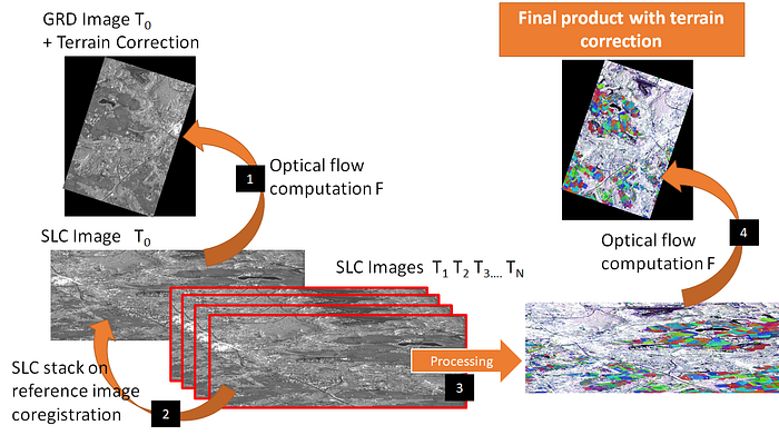
In this post, we’ll deal only with the second point: how to calculate the displacement (assumed to be bijective) between two images of the same dimensions.
Note that in the case of radar time series, we can often hesitate between:
- georeference/orthorectify all images, then compensate for residual displacements at the end of these steps
- or re-align all images to a reference image, process the re-aligned series, then georeference/orthorectify the result. I prefer the latter solution, as it makes it easier to retain phase information while respecting the original sampling. In this case, to georeference the result, we can simply georeference the reference image, retain the transformation result, and apply it to all images in the rectified series. The terrain rectification step can be envisaged as a recalibration between the reference image of the series, and the Sentinel-1 image of the same footprint after orthorectification (available in most current platforms).
The main types of methods for calculating deformation between two images
Geometric calculation
When two radar images need to be recalibrated, it is always possible to retrieve fine information relying on precise knowledge of the satellite’s orbital parameters and the terrain’s topography. These are purely “geometric” approaches. On the other hand, they require a thorough knowledge of the DEM, the trajectories used to form the images, and how to access them. In the case of airborne data, challenges arise, particularly when dealing with potentially inaccurate trajectory data.
Frequently, deformation calculations are limited to specific points within the image, typically referred to as Ground Control Points (GCPs).
Calculating displacement from images
In this case, deformations are calculated solely on the basis of the information contained in the images, without any auxiliary data or metadata.
This category of algorithms can be aptly compared with motion estimation: the process of studying the movement of objects in a video sequence, looking for correlation between two successive images in order to predict the change in position of the content.
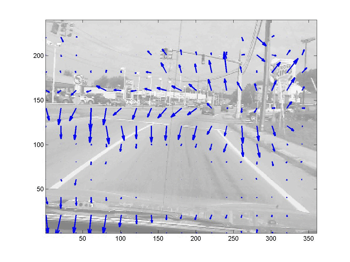
There are several methods of motion estimation, the best-known being Block-Matching and Optical Flow, with Block-Matching operating on block small images extracted from the overall image, and Optical Flow taking into account the entire image.
Optical flow methods have been considered for remote sensing in [Gefolki] (see bibliography)
However, in contemporary applications, deep learning offers two noteworthy capabilities:
- either the selection of precise and reliable correspondence points between the two images.
- or the direct computation of motion functions through supervised learning.
In a subsequent post, we will delve into the contemporary uses of deep learning architectures for these functions.
How do you visualize a motion field, and the effectiveness of registration?
In Computer Vision, we usually represent a displacement flow with an HSV palette whose color codes the orientation, and whose luminance codes the norm of the displacement vector, as follows:
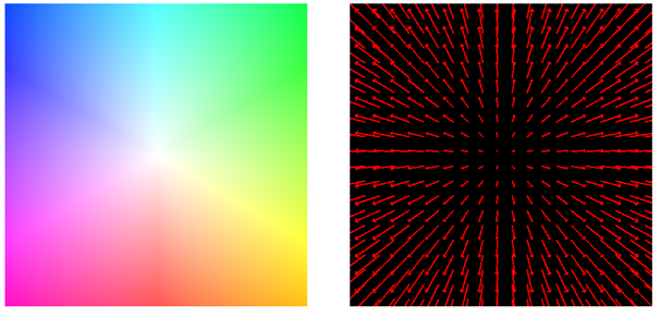
if you know the flow/deformation you wish to find, it’s easy enough to consider the algorithm’s errors by observing the differences in norm and orientation of the vectors found.
On the other hand, if you have no idea what to expect, you need to compare the image pairs before and after resampling the secondary image on the reference image, having corrected the flow.
This can be done :
- by making mosaics of images

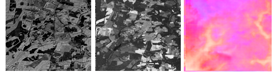
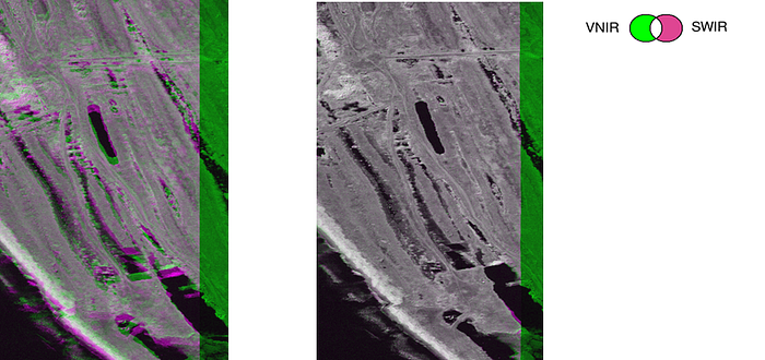
- by creating colorful compositions in complementary colors.
In this case, coregistration faults appear at the colored borders.
- by making a small animated gif of the images after correction to check that they overlap well.
They are qualitative visualization.
To go a step further, and get a more quantitative analysis, we really have no choice but to check the good concordance of points or salient features such as segments, in the two images.
Bottom line:
● coregistration is used to combine information from several images in the same area● motion estimation or flow estimation can be used as a central building block for coregistration — now deep learning methods exist to this aim.
● image georeferencing resampling has an impact on the final result; care must be taken when performing this step, preferably at the end of processing.
● to assess the quality of a deformation estimate, several alternatives exist (colored superposition, animation, mosaic) — a quantitative estimate requires more steps.
Bibliography: classical optical flow for remote sensing image registration
Brigot, G., et al. (2016). Adaptation and evaluation of an optical flow method applied to coregistration of forest remote sensing images. IEEE Journal of Selected Topics in Applied Earth Observations and Remote Sensing, 9(7), 2923–2939.
Plyer, A., et al. (2015). A new coregistration algorithm for recent applications on urban SAR images. IEEE Geoscience and Remote Sensing Letters, 12(11), 2198–2202.
