How to evaluate detection performance…with object or pixel approaches?
As we’ve already seen in this post, in general the computer vision field has an “object” type approach, while other approaches in the remote sensing field work very much with “pixel” type algorithms.
This sometimes leads to far-fetched discussions about “which performance curves should I calculate”, are they comparable?
Here I address this question for the detection functionality
Spoiler Alert: No, you can’t directly compare the performance curves of pixelwise and object detection approaches.
Here, I propose to start with an example of objects to be detected in an image: buildings.
First step: what is my detection product, what is my ground truth?
To define most performance criteria, we need the notion of “Positive” in what we DETECT.
In the pixel approach, “POSITIVES” are pixels set to 1 in my detection result. In the “object” approach, the “Positives” are the boxes we’ve found.

Now let’s look at the “ground truth”, the ultimate Grail towards which we want to converge. Ground truth can correspond to several types of product:

Remember that raster data is information given as images, while vector data are lists (or vectors) of geometric elements: points or polygons, with their coordinates.
Only in the case of raster data do you immediately have something usable with a pixel detection result. Otherwise, if I have vector data and image data on one side, I need to “rasterize” (transform into an image) my vector data.
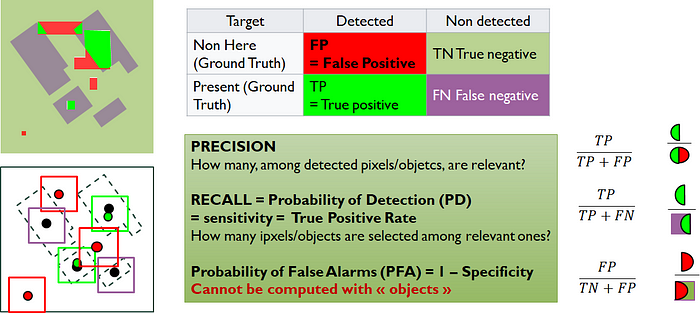
Once I have a ground truth and a detection result, my task will be to compare the two, and to do this I’ll define “True positives”, “True Negatives”, “False Positives” and “False Negatives”.
Define True positive, False positive, etc.
The pixel case
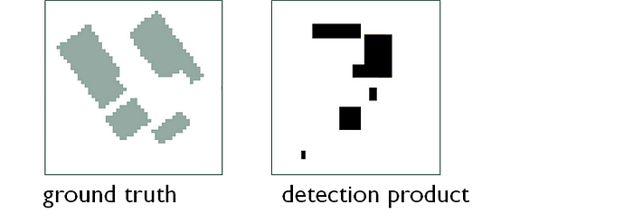
This is the simplest case. We always start with the same example: on the left, my ground truth, on the right: what I detected (and yes, my result really sucks).

It’s simply a matter of counting :
- my True Positives: my detected pixels that are actually on the Ground Truth.
- my False Positives: my detected pixels that are not on the Ground Truth.
Then consider the remaining pixels, the negatives:
- my False Negatives: the pixels I didn’t detect when I should have!
- my True Negatives: the pixels I didn’t detect, and so much the better.

The object Case
This case is far more ambiguous, and presents several difficulties:
- firstly, the true positive must be defined according to certain criteria. For example, if I’ve detected a building, but it’s not exactly in the right place, does it count as a true positive or not?
Generally speaking, we define the true positive “as we see fit”, with the possibility of leaving ourselves a margin of error in terms of position, etc. Take the example of the green boxes on the left, which count as “True” even though they are slightly offset from the VT.

- second difficulty: it’s not really possible to define the notion of “True Negative”. Because the background is not made up of a countable set of objects!
Precision, Recall, False Alarms…
From there, there are several parameters for measuring performance. To make matters worse, some words are redundant in the literature.
- precision. It is useful for checking that you’re not messing around.
- recall = probability of detection = sensitivity = True positive Rate.
- Probability of False Alarm= 1-specificity
Useful if you don’t want to have a flashing Christmas tree in a detection map where you’re looking for rare things.

Warning: it makes no sense to display only one of these performance parameters!
I’ve seen it all before: “we’re too good, we display a detection probability of 100%”.
Yes, me too, all I have to do is to decide that all my pixels are a detection.
Let’s say my image contains N pixels, and that my buildings cover M pixels of the image in the Ground Truth. In this case :
TP= M, FN=0, TN=0, FP=(N-M).
My accuracy is equal to M/N…(which doesn’t really depend on me, but only on the density of buildings to be detected…)…
But where it really gets tricky is that the probability of a false alarm is 1. That’s a bit of a game-changer, isn’t it?
Performance curves
So, if it’s “wrong” to consider only one parameter, we like to consider duos, and establish “performance curves”. In detection, these are of two types:
- Receiver Operating Characteristic curve, or ROC curve
- Precision / Recall or or PR curve
Let’s see what they look like:

The first is generally preferred for detection tasks, especially in medicine (we don’t like having false diagnoses such as “you have a serious disease” when it’s not true).
BUT it’s rarely seen in “object” approaches. Simply because we can’t define a “false non-detection” very well, and there’s no definition of background objects.
In contrast, computer vision approaches fall back on precision-recall curves. This is possible because it will not contain the definition of false alarm.
Finally, if defined in pixel terms, these curves have certain charming properties of monotonicity.
Introducing acceptance margins into the definition of a true positive will introduce bias into these properties. And sometimes this leads to rather bizarre behavior in the curves…
In a nutshell
Each case-study calculates true negatives /positives in its own way, in terms of:
- shape overlap
- distance between bounding boxes
- number of pixels detected, etc.
A ROC curve includes the “true negatives” (or the “background” surface). A Precision/Recall don’t.
In the “object” approach, defining a true negative doesn’t make sense.
It is therefore not possible to calculate a ROC curve with an object approach.
For classification problems, precision-recall curves can be generalized to each class.
My feeling is that a problem that is a single-class classification is called detection, whereas the specific notions of detection don’t generalize well to the case of object classification.
To go further:
Davis, J., & Goadrich, M. (2006, June).
The relationship between Precision-Recall and ROC curves.
In Proceedings of the 23rd international conference on Machine learning (pp. 233–240):
● Receiver Operator Characteristic (ROC) curves are commonly used for binary decision (detection) problems in machine learning.
● When dealing with highly skewed datasets, when you care more about the rare case (classification), Precision-Recall (PR) curves are informative on algorithm’s performance.
● A curve dominates in ROC space if and only if it dominates in PR space.
● It is incorrect to linearly interpolate between points in Precision-Recall space.
● Algorithms that optimize the area under the ROC curve are not guaranteed to optimize the area under the PR curve.
