From Correlation to Contrast: How partially correlated Speckle Intensities Behave in Coherent Imaging
Skipping the Equations — Here’s What You Need!
Have you ever wondered how the contrast D between two speckle images X and Y evolves when these images share a certain level of correlation?

How does that contrast behave when dealing with two SAR (radar) backscatter images, two polarimetric channels, or even dynamic laser speckle images where we get multiple speckle acquisitions over time?
These questions are at the heart of understanding correlated intensity fluctuations in coherent imaging systems, and they motivate the study of how two intensity patterns, drawn from correlated speckle fields, compare to one another.
In this post, I’ll walk you through the key ideas of a recent preprint (available on arXiv: https://arxiv.org/pdf/2503.08808 ) focusing on why the correlation matters and what the properties of the contrast |X-Y|/(X+Y) are.
Mathematical derivations are described in the paper. Here I’ll highlight the conceptual steps and the main take-home results.
What’s Speckle and Why Correlation Matters
Speckle patterns arise whenever coherent waves (optical, radar, or ultrasound) reflect or scatter from rough surfaces or random media. If you illuminate a rough surface with a laser, or probe the Earth’s surface with a coherent radar signal, the scattered fields interfere in seemingly random ways, forming a “speckle” pattern of bright and dark spots. When we measure speckle intensity, we often model it statistically:
- Single-look intensity is commonly represented by an exponentially distributed random variable.
- Multi-look intensity (where several independent speckles are summed or averaged) often follows a Gamma distribution.
Real systems frequently involve two or more speckle images (e.g., different polarimetric channels, different radar acquisitions, or multiple time frames in dynamic speckle imaging). In these scenarios, the intensities may not be independent: a certain degree of correlation can persist between the measurements. Our goal is to quantify how the contrast D between the two images depends on the correlation level and the Equivalent Number of Looks (ENL).
The Modeling Approach: From Circular Gaussians to Gamma Intensities
Starting Point: Circular Complex Gaussian Fields
One elegant way to handle speckle mathematically is to start with two circular (or “circularly symmetric”) complex Gaussian random fields:
Z1, Z2 with zero mean, same variance, and correlation ρ
In such fields, each Zi is a complex-valued variable whose real and imaginary parts are jointly Gaussian with equal variance. The core parameter here is the field correlation coefficient, say ρ, which captures how much Z1 and Z2 are close together.
Intensities and Correlation
When we measure intensity, we look at |Zk|². Indeed, if the complex fields have correlation coefficient ρ, one finds that the intensities X=|Z1|² and Y=|Z2|² typically end up with correlation |ρ|².
That means that the correlation in the underlying complex fields translates to a lower correlation in their intensities.
Multilook or Summation: From Exponential to Gamma
A single speckle intensity is (in the simplest, fully developed regime) exponentially distributed. But in practice, we often integrate or sum multiple “looks”:
- In radar, that could be k looks for noise-reduction purposes.
- In optics, that could be k grains of speckle integrated during a given period if the scatterers are moving.
Summing k independent exponential random variables yields a Gamma distribution with shape parameter k. Hence, if each look stems from correlated exponential variables, we end up with two correlated Gamma variables X and Y.
A Useful Contrast Measure: D(X,Y)=|X-Y|/(X+Y)
To compare the intensities X and Y, we introduce the normalized contrast (sometimes called the Fujii index in dynamic speckle contexts):
This quantity:
- Lies between 0 and 1.
- Equals 0 when X≈Y.
- Increases toward 1 when X and Y differ substantially.
Because D is scale-invariant — multiplying X and Y by a positive constant leaves D unchanged — it nicely captures how dissimilar the two intensities are, irrespective of absolute brightness.
Key Results
In the preprint, we show (through a series of variable transformations and integral identities) that the probability distribution of D can be derived in closed form when X and Y are correlated Gamma variables with shape parameter k and correlation ρ (k reflects the number of looks or number of speckle grains summed) :

B is the Beta function.
Besides the full probability distribution, one can also compute the moments of D of any order m. Three formulations exist. All these moment formulas appear in closed form as hypergeometric functions F, which modern software libraries (e.g., Python’s scipy.special) can evaluate easily.
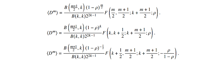
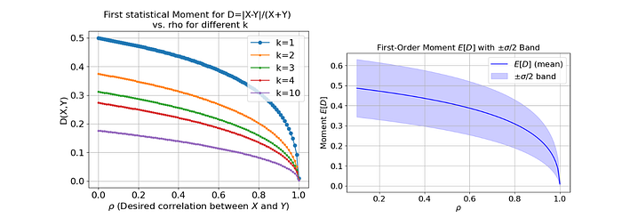
For instance, the mean of D is a quick one-number summary:
- When ρ=0 and k=1, the mean value of D is 1/2, reflecting that completely uncorrelated, single-look intensities give a wide spread in values centered around 1/2.
- As ρ→1, the mean of D drops toward 0.
- As k increases, the mean (and higher-order moments) typically shrink, showing that multi-look averaging “smooths out” fluctuations.
Potential Applications
Why does this matter in practice? Here are a few scenarios:
- Radar Imaging (Multi-look Intensity)
In synthetic aperture radar (SAR), multi-look techniques average independent “looks” to reduce noise. If we have two correlated SAR images (e.g., from slightly shifted acquisitions or different polarizations), analyzing D helps us see how different they are while factoring out their overall brightness. - Dynamic Speckle for Slow Motion Detection
In laser speckle contrast imaging, you track speckle patterns over time to detect small motions in complex systems. If the motion is very slow (e.g. sap flow), the speckle fields remain highly correlated from one frame to the next, so D is near zero. Small changes in D can be surprisingly sensitive in highlighting very small motions. It is known as the Fujii index in the literature of biospeckle. - Dynamic Speckle for Rapid Motion Detection
When motion in a medium accelerates — such as blood flow in biological tissues — the speckle field decorrelates rapidly, reducing the correlation coefficient ρ toward zero. Over a typical exposure time, the detector then integrates an increasing number of speckle grains, which corresponds to a larger shape parameter k. Consequently, fluctuations in measured intensity are averaged out, lowering the observed speckle contrast D:

A fully functional Google Colab notebook (Python) is available for anyone interested in exploring all the numerical simulations and empirical checks of the derived distributions and moments. You can access it here: Google Colab Link.
Please if this is useful for you, cite:
Distribution and Moments of a Normalized Dissimilarity Ratio for two Correlated Gamma Variables, Elise Colin and Razvigor Ossikovski, 2025, arXiv 2503.08808, https://arxiv.org/abs/2503.08808}
